Optimize Projects Using the Performance Tab
Efficient projects are extremely important in production, the less time you spend investigating issues, the more time you can spend on look development or lighting. The Performance tab helps you understand where bottlenecks may lie in your node graph by interpreting profiling information.
You can see at glance how many nodes you have in the recipe, how many are contributing to your scene, and which nodes use more CPU resources. The Heat Map allows you to view this information directly in the Node Graph tab, providing a visual indication of expensive nodes so you can debug scenes more effectively.
If you're still not sure where optimizations can improve your scene, you can send the Profile Results File to a colleague for analysis. Profiling data is automatically saved as .json files to the KATANA_TMPDIR location.
Tip: The .json location is also recorded in the Render Log if you're not sure where the file is saved. See Renderer Logging for more information.
Analyze the Scene with the Performance Tab
- Load the project you want to analyze and optimize.
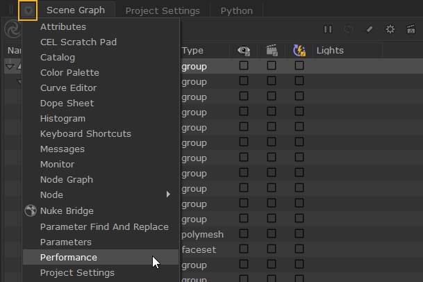
- Navigate to the Performance tab or click the Add Tab button and then select Performance if the tab is not already in your workspace.
- Select and deselect nodes in the node graph to update the Number of Selected Nodes indicator. The number in brackets indicates nodes that are not visible at the root level, such as those in groups and super tools.
The Performance tab is added to the pane and the Project Stats displays the number of nodes in the scene and how many of those nodes are contributing.
The Number of Nodes and Contributing Nodes listed includes all nodes inside groups, Network Material contexts, and super tools such as Gaffer3. As a result, the number may be higher than looking at the node graph suggests.
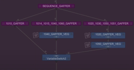
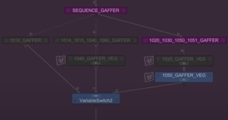
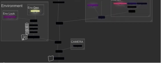
To see a visual representation of contributing nodes, go to View > Dim Nodes Not Contributing to Viewed Node. Nodes that are not contributing are dimmed.
|
|
|
|
All nodes appear to be contributing |
Non-contributing nodes are dimmed |
To display more in-depth data
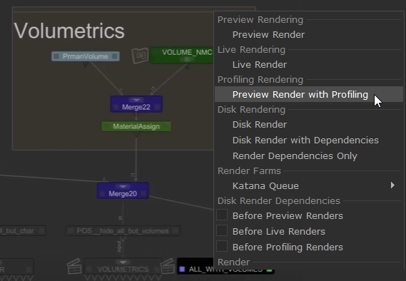
- Render the scene from any node by right-clicking the node and selecting Preview Render with Profiling.
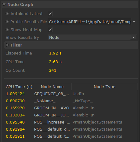
- The Performance tab shows the time to first pixel rendered and a list of nodes and CPU usage, with the most expensive nodes at the top. As you can see in this example, importing geometry (UsdIn) and merging (Merge) are quite CPU-heavy operations.
- Enable Show Heat Map to display heat colors in the Node Graph tab.
- If you have difficulty distinguishing between nodes with similar color gradients, you can change the heat map color scheme by clicking View > Heat Color Map and selecting a new scheme. For example, Magma colors cheap nodes black, which can be easily ignored.
Note: The _NoName_ entry represents all operations that are not related to nodes, such as implicit resolvers. See Implicit Resolvers for more information.
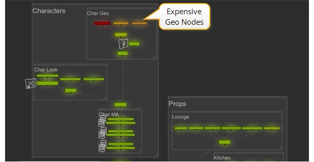
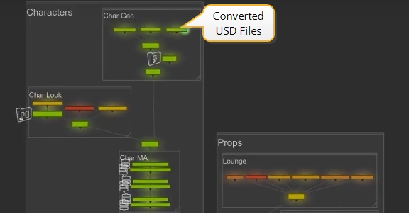
In this example, the Char Geo import nodes are clearly the most expensive nodes.
Tip: There's also colored scale at the bottom-left of the Node Graph tab that displays color against a relative CPU time value. The range adjusts dynamically between the least expensive node and most expensive node, which allows it to scale to any size of project.
Utilizing the Filtering Options
Once you start using the Performance tab more extensively, you might need to start filtering the results seen. As important it is to know which nodes are the most expensive, you might want to hide away certain names or types.
One example of why you might want to do this, is when specific nodes may naturally have a high cook time result. For example, nodes which are referencing geometry (e.g. the UsdIn) may display the highest CPU Time in the list, but it’s sometimes not an area that will require any optimization. Narrowing down the search to focus on areas that will need that attention is therefore more useful when optimizing Katana projects.
Options for filtering can be found in the Performance tab under Node graph > Filter.
• Show Results - adjusts the number of results being shown in the list, by default this will be set to 20
• Node Name and Node Type pages will be available, as well as Op Name and Op Type pages (when Show Results By is set to Ops) - all of which include two entries:
• Include Only - Will take in a list to only include results that match the conditions specified
• Exclude - Will take a list to exclude results that match the conditions specified
Expression matching for these fields are as follows:
|
Pattern |
Meaning |
|---|---|
| * | Matches everything |
|
? |
Matches any single character |
|
[seq] |
Matches any character in seq |
|
[!seq] |
Matches any character not in seq |
Tip: You can use either commas and spaces in order to separate the patterns specified in these fields
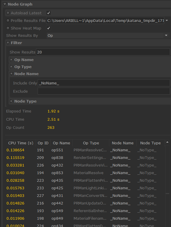
In the example below, we have set a filter for the _NoName_ entry, in order to delve into operations unrelated to nodes, such as implicit resolvers. See Implicit Resolvers for more information. For those wanting a breakdown of these _NoName_ operations, it is possible to set the Show Results By field to Ops, in order to view a breakdown of these implicit resolvers.
Optimizing Nodes with the Heat Map
Katana's Performance tab heat map gives you a breakdown of your entire project at a glance. It's easy to locate CPU-heavy nodes so you can investigate where performance can be improved.
- Render the scene by right-clicking a render node and selecting Preview Render with Profiling.
- The Performance tab shows the time to first pixel rendered and a list of nodes and CPU usage, with the most expensive nodes at the top.
- Enable Show Heat Map to display heat colors in the Node Graph tab.
In this example, the Char Geo import nodes are clearly the most expensive nodes.
Geometry nodes are often CPU-heavy, but in this case we've imported USD files that were encoded as .usda, which is not an optimal format for character animation.
In this particular case, the way we have reduced CPU time is to convert the data into .usd files, which subsequently made the time against those geometry nodes more efficient. If we then recalculate the Node Graph data in the Performance tab, we get a much more varied heat map. This is because the UsdIn nodes are no longer using way more resources that all other nodes, which evens out the heat map colors.
Note: Subsequent profile .json files don’t overwrite each other, you get a new file for each calculation with a time stamp.
This is a very simple example, but it highlights the power of the heat map for locating bottlenecks in your Katana projects.
Phone a Friend if You Can’t Troubleshoot Yourself
OK, so you've removed bottlenecks and reduced some of the CPU-heavy nodes' processing time, but your project is still not as optimal as it could be. Time to call for help. Katana saves performance data to Profile Results Files automatically, which you can share with colleagues if you're really stuck. Your colleague only needs your Katana project and your profile .json file to get started, they don't even have to perform a render because all the data they need is already in the .json file.
Note: If changes are made in the scene, the imported static profiling data becomes invalid. You'll need to run another Preview Render with Profiling to update the data to include any changes.
Profiling data is automatically saved as .json files to the KATANA_TMPDIR location, but you can specify a different directory at startup using the --profiling-dir command line argument. See Command-line Interface for more information.
- Save the project and make a note of the Profile Results File location. Send the project and the .json file to your colleague.
- On their machine, load the Katana project and open the Performance tab.
- In the Profile Results File field, enter the location of the profiling .json or click the Browse dropdown to navigate to the location of the file.
- Enable Show Heat Map, if it isn't already checked.
They don’t need to execute the Preview Render with Profiling step themselves, the data is already available.
All the data is now available for your colleague to help you get back on track.